Range only SLAM, Singular – i.e. "Under-Constrained"
Keywords: underdetermined, under-constrained, range-only, singular
This tutorial describes a range-only system where there are always more variable dimensions than range measurements made. The error distribution over ranges could be nearly anything, but are restricted to Gaussian-only in this example to illustrate an alternative point – other examples show inference results where highly non-Gaussian error distributions are used.
Presentation Style Discussion
A presentation discussion of this example is available here:
Towards Real-Time Non-Gaussian SLAM from Dehann on Vimeo.
A script to recreate this example is provided in RoME/examples here. This singular range-only illustration:
Multi-modal iSAM range and distance only example from Dehann on Vimeo.
Quick Install
If you already have Julia 1.0 or above, alternatively see complete installation instructions here:
julia> ]
(v1.0) pkg> add RoME, Distributed
(v1.0) pkg> add RoMEPlotting
The Julia REPL/console is sufficient for this example (copy-paste from this page). Note that more involved work in Julia is simplified by using the Juno IDE.
Note A recent test (May 2019, IIF v0.6.0) showed a possible bug was introduced with one of the solver upgrades. THe figures shown on this example page are still, however, valid. Previous versions of the solver, such as IncrementalInference v0.4.x and v0.5.x, should still work as expected. Follow progress on issue 335 here as bug is being resolved. Previous versions of the solver can be installed with the package manager, for example:
(v1.0) pkg> add IncrementalInference@v0.5.7. Please comment for further details.
Loading The Data
Starting a Juno IDE or Julia REPL session, the ground truth positions for vehicle positions GTp and landmark positions GTl can be loaded into memory directly with these values:
GTp = Dict{Symbol, Vector{Float64}}()
GTp[:l100] = [0.0;0]
GTp[:l101] = [50.0;0]
GTp[:l102] = [100.0;0]
GTp[:l103] = [100.0;50.0]
GTp[:l104] = [100.0;100.0]
GTp[:l105] = [50.0;100.0]
GTp[:l106] = [0.0;100.0]
GTp[:l107] = [0.0;50.0]
GTp[:l108] = [0.0;-50.0]
GTp[:l109] = [0.0;-100.0]
GTp[:l110] = [50.0;-100.0]
GTp[:l111] = [100.0;-100.0]
GTp[:l112] = [100.0;-50.0]

GTl = Dict{Symbol, Vector{Float64}}()
GTl[:l1] = [10.0;30]
GTl[:l2] = [30.0;-30]
GTl[:l3] = [80.0;40]
GTl[:l4] = [120.0;-50]
NOTE 1. that by using location indicators :l1, :l2, ... or :l100, :l101, ... is of practical benefit when visualizing with existing RoMEPlotting functions.
NOTE 2. Landmarks must be in range before range measurements can be made to them.
Creating the Factor Graph with Point2
The first step is to load the required modules, and in our case we will add a few Julia processes to help with the compute later on.
# add more julia processes
using Distributed
nprocs() < 4 ? addprocs(4-nprocs()) : nothing

# tell Julia that you want to use these modules/namespaces
using RoME
NOTE Julia uses just-in-time compiling (unless pre-compiled), therefore each time a new function call on a Julia process will be slow, but all following calls to the same functions will be as fast as the statically compiled code.
This example exclusively uses Point2 variable node types, which have dimension 2 and represent [x, y] position estimates in the world frame.
Next construct the factor graph containing the first pose :l100 (without any knowledge of where it is) and three measured beacons/landmarks :l1,:l2,:l3 – with prior location knowledge for :l1 and :l2:
# create the factor graph object
fg = initfg()

# first pose with no initial estimate
addVariable!(fg, :l100, Point2)

# add three landmarks
addVariable!(fg, :l1, Point2)
addVariable!(fg, :l2, Point2)
addVariable!(fg, :l3, Point2)

# and put priors on :l101 and :l102
addFactor!(fg, [:l1;], PriorPoint2(MvNormal(GTl[:l1], diagm(ones(2)))) )
addFactor!(fg, [:l2;], PriorPoint2(MvNormal(GTl[:l2], diagm(ones(2)))) )
The PriorPoint2 is assumed to be a multivariate normal distribution of covariance diagm(ones(2)). Note the API PriorPoint2(::T) where T <: SamplableBelief = PriorPoint2{T} to accept distribution objects, discussed further in subsection Various SamplableBelief Distribution Types.
Adding Range Measurements Between Variables
Next we connect the three range measurements from the vehicle location :l0 to the three beacons, respectively – and consider that the range measurements are completely relative between the vehicle and beacon position estimates:
# first range measurement
rhoZ1 = norm(GTl[:l1]-GTp[:l100])
ppr = Point2Point2Range( Normal(rhoZ1, 2) )
addFactor!(fg, [:l100;:l1], ppr)

# second range measurement
rhoZ2 = norm(GTl[:l2]-GTp[:l100])
ppr = Point2Point2Range( Normal(rhoZ2, 3.0) )
addFactor!(fg, [:l100; :l2], ppr)

# second range measurement
rhoZ3 = norm(GTl[:l3]-GTp[:l100])
ppr = Point2Point2Range( Normal(rhoZ3, 3.0) )
addFactor!(fg, [:l100; :l3], ppr)
The ranging measurement standard deviation of 2.0 or 3.0 is taken, assuming a Gaussian measurement assumption. Again, any distribution could have been used. The factor graph should look as follows:
drawGraph(fg) # show the factor graph
Inference and Visualizations
At this point we can call the solver start interpreting the first results:
tree = solveTree!(fg)The factor graph figure above showed the structure between variables and factors. In order to see the numerical values contained in the factor graph, a set of tools are provided by the RoMEPlotting and KernelDensityEstimatePlotting packages. For more details, please see the dedicated visualization discussion here.
First look at the two landmark positions :l1, :l2 at (10.0,30),(30.0,-30) respectively.
using RoMEPlotting

plotKDE(fg, [:l1;:l2], dims=[1;2])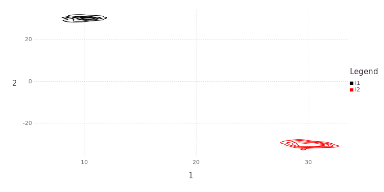
Similarly, the belief estimate for the first vehicle position :l100 is bi-modal, due to the intersection of two range measurements:
plotKDE(fg, :l100, dims=[1;2], levels=6)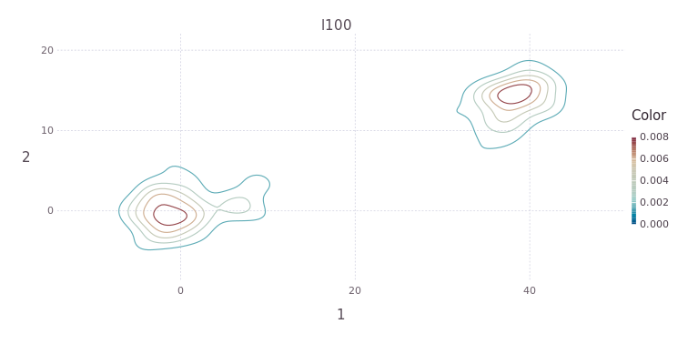
An alternative plotting interface can also be used, that shows a histogram of desired elements instead:
drawLandms(fg, from=1, to=101, contour=false, drawhist=true)
Notice the ring of particles which represents the belief on the third beacon/landmark :l3, which was not constrained by a prior factor. Instead, the belief over the position of :l3 is being estimated simultaneous to estimating the vehicle position :l100.
Implicit Growth and Decay of Modes (i.e. Hypotheses)
Next consider the vehicle moving a distance of 50 units–-and by design the direction of travel is not known–-to the next true position. The video above gives away the vehicle position with the cyan line, showing travel in the shape of a lower case 'e'. The following function handles (pseudo odometry) factors as range-only between positions and range-only measurement factors to beacons as the vehice travels.
function vehicle_drives_to!(fgl::G, pos_sym::Symbol, GTp::Dict, GTl::Dict; measurelimit::R=150.0) where {G <: AbstractDFG, R <: Real}
  currvar = union(ls(fgl)...)
  prev_sym = Symbol("l$(maximum(Int[parse(Int,string(currvar[i])[2:end]) for i in 2:length(currvar)]))")
  if !(pos_sym in currvar)
    println("Adding variable vertex $pos_sym, not yet in fgl<:AbstractDFG.")
    addVariable!(fgl, pos_sym, Point2)
    @show rho = norm(GTp[prev_sym] - GTp[pos_sym])
    ppr = Point2Point2Range( Normal(rho, 3.0) )
    addFactor!(fgl, [prev_sym;pos_sym], ppr)
  else
    @warn "Variable node $pos_sym already in the factor graph."
  end
  beacons = keys(GTl)
  for ll in beacons
    rho = norm(GTl[ll] - GTp[pos_sym])
    # Check for feasible measurements:  vehicle within 150 units from the beacons/landmarks
    if rho < measurelimit
      ppr = Point2Point2Range( Normal(rho, 3.0) )
      if !(ll in currvar)
        println("Adding variable vertex $ll, not yet in fgl<:AbstractDFG.")
        addVariable!(fgl, ll, Point2)
      end
      addFactor!(fgl, [pos_sym;ll], ppr)
    end
  end
  nothing
end
After pasting (or running) this function in Julia, a new member definition vehicle_drives_to! can be used line any other function. Julia will handle the just-in-time compiling for the type specific function required and cach the static code for repeat executions.
NOTE The exclamation mark at the end of the function name has no syntactic significance in Julia, since the full UTF8 character set is available for functions or variables. Instead, the exclamation serves as a Julia community convention to tell the caller that this function will modify the contents of at least some of the variables being passed into it – in this case the factor graph
fgwill be modified.
Now the actual driving event can be added to the factor graph:
#drive to location :l101, then :l102
vehicle_drives_to!(fg, :l101, GTp, GTl)
vehicle_drives_to!(fg, :l102, GTp, GTl)

# see the graph
drawGraph(fg, engine="neato")
NOTE The distance traveled could be any combination of accrued direction and speeds, however, a straight line Gaussian error model is used to keep the visual presentation of this example as simple as possible.
The marginal posterior estimates are found by repeating inference over the factor graph, followed drawing all vehicle locations as a contour map:
# solve and show message passing on Bayes (Junction) tree
getSolverParams(fg).drawtree=true
getSolverParams(fg).showtree=true
tree = solveTree!(fg)

# draw all vehicle locations
pl = plotKDE(fg, [Symbol("l$(100+i)") for i in 0:2], dims=[1;2])
# Gadfly.draw(PDF("/tmp/testL100_102.pdf", 20cm, 10cm),pl) # for storing image to disk

pl = plotKDE(fg, [:l3;:l4], dims=[1;2], levels=4)
# Gadfly.draw(PNG("/tmp/testL3_4.png", 20cm, 10cm),pl)
Notice how the vehicle positions have two hypotheses, one left to right and one diagonal right to bottom left – both are valid solutions!
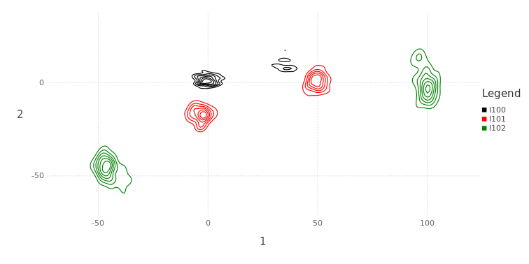
The two "free" beacons/landmarks :l3,:l4 still have several modes each, implying insufficient data to constrain either to a strong unimodal belief.

vehicle_drives_to!(fg, :l103, GTp, GTl)
vehicle_drives_to!(fg, :l104, GTp, GTl)

tree = solveTree!(fg)

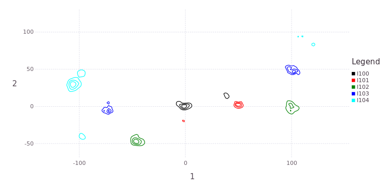
pl = plotKDE(fg, [Symbol("l$(100+i)") for i in 0:4], dims=[1;2])
# Gadfly.draw(PDF("/tmp/testL100_104.pdf", 20cm, 10cm),pl)
Moving up to position :l104 still shows strong multiodality in the vehicle position estimates:
vehicle_drives_to!(fg, :l105, GTp, GTl)
vehicle_drives_to!(fg, :l106, GTp, GTl)

tree = solveTree!(fg)


vehicle_drives_to!(fg, :l107, GTp, GTl)

tree = solveTree!(fg)


vehicle_drives_to!(fg, :l108, GTp, GTl)

tree = solveTree!(fg)


pl = plotKDE(fg, [Symbol("l$(100+i)") for i in 2:8], dims=[1;2], levels=6)
# Gadfly.draw(PDF("/tmp/testL103_108.pdf", 20cm, 10cm),pl)
Next we see a strong return to a single dominant mode in all vehicle position estimates, owing to the increased measurements to beacons/landmarks as well as more unimodal estimates in :l3, :l4 beacon/landmark positions.
vehicle_drives_to!(fg, :l109, GTp, GTl)
vehicle_drives_to!(fg, :l110, GTp, GTl)

tree = solveTree!(fg)


vehicle_drives_to!(fg, :l111, GTp, GTl)
vehicle_drives_to!(fg, :l112, GTp, GTl)

tree = solveTree!(fg)


pl = plotKDE(fg, [Symbol("l$(100+i)") for i in 7:12], dims=[1;2])
# Gadfly.draw(PDF("/tmp/testL106_112.pdf", 20cm, 10cm),pl)

pl = plotKDE(fg, [:l1;:l2;:l3;:l4], dims=[1;2], levels=4)
# Gadfly.draw(PDF("/tmp/testL1234.pdf", 20cm, 10cm),pl)

pl = drawLandms(fg, from=100)
# Gadfly.draw(PDF("/tmp/testLocsAll.pdf", 20cm, 10cm),pl)
Several location belief estimates exhibit multimodality as the trajectory progresses (not shown), but collapses and finally collapses to a stable set of dominant position estimates.

Landmark estimates are also stable at one estimate:

In addition, the SLAM 2D landmark visualization can be re-used to plot more information at once:
# pl = drawLandms(fg, from=100, to=200)
# Gadfly.draw(PDF("/tmp/testLocsAll.pdf", 20cm, 10cm),pl)

pl = drawLandms(fg)
# Gadfly.draw(PDF("/tmp/testAll.pdf", 20cm, 10cm),pl)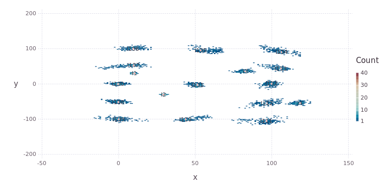
This example used the default of N=200 particles per marginal belief. By increasing the number to N=300 throughout the test many more modes and interesting features can be explored, and we refer the reader to an alternative and longer discussion on the same example, in Chapter 6 here.