Visualization with Arena.jl
Caesar.jl uses the Arena.jl package for all the visualization requirements. This part of the documentation discusses the robotic visualization aspects supported by Arena.jl. Arena.jl supports a wide variety of general visualization as well as developer visualization tools more focused on research and development.
Current Work In Progress
Written Nov 2018
While Arena.jl is still being upgraded for Julia 1.0 (mostly relating to updates in 3D visualization), the 2D visualizations available through the development master branch in RoMEPlotting.jl are available in Julia 1.0. The master branch version can be installed using the Julia package manager with add RoMEPlotting#master, see also environment installation page.
Introduction
Over time, Caesar.jl has used a least three different 3D visualization technologies, with the most recent based on WebGL and three.js by means of the MeshCat.jl package. The previous incarnation used a client side installation of VTK by means of the DrakeVisualizer.jl and Director libraries. Different 2D plotting libraries have also been used, with evolutions to improve usability for a wider user base. Each epoch has aimed at reducing dependencies and increasing multi-platform support.
The sections below discuss 2D and 3D visualization techniques available to the Caesar.jl robot navigation system. Visualization examples will be seen throughout the Caesar.jl package documentation. Arena.jl is intended to simplify the process 2D plotting for robot trajectories in two or three dimensions. The visualizations are also intended to help with subgraph plotting for finding loop closures in data or compare two datasets.
Note that all visualizations used to be part of the Caesar.jl package itself, but was separated out to Arena.jl in early 2018.
Installation
MeshCat / three.js Viewer (WebGL)
For the 3D visualization tools provided for Caesar.jl–-in a Julia or (JuliaPro) terminal/REPL–-type ] to activate pkg manager and install Arena the master branch
(v1.0) pkg> add Arena#masterCurrent master branch development allows the user to use the three.js WebGL based viewer via MeshCat.jl.
2D Visualization
2D plot visualizations, provided by [RoMEPlotting.jl(http://www.github.com/JuliaRobotics/RoMEPlotting.jl) and KernelDensityEstimatePlotting.jl, are generally useful for repeated analysis of a algorithm or data set being studied. These visualizations are often manipulated to emphasize particular aspects of mobile platform navigation.
Install RoMEPlotting master branch:
(v1.0) pkg> add RoMEPlotting#masterInteractive Gadfly.jl Plots
See the following two discussions on Interactive 2D plots:
Hexagonal 2D SLAM example visualization
The major 2D plotting functions between RoMEPlotting.jl:
drawPosesdrawPosesLandmsdrawSubmaps
and KernelDensityEstimatePlotting.jl:
plotKDE/plot(::KernelDensityEstimate)
This simplest example for visualizing a 2D robot trajectory–-such as first running the Hexagonal 2D SLAM example–-
# Assuming some fg::FactorGraph has been loaded/constructed
# ...

using RoMEPlotting

# For Juno/Jupyter style use
pl = drawPosesLandms(fg)

# For scripting use-cases you can export the image
Gadfly.draw(PDF("/tmp/test.pdf", 20cm, 10cm),pl)  # or PNG(...)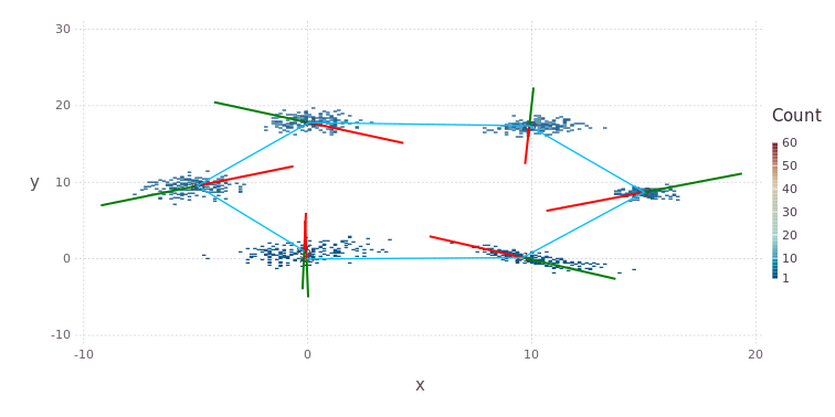
Density Contour Map
KernelDensityEstimatePlotting (as used in RoMEPlotting) provides an interface to visualize belief densities as counter plots. The following basic example shows some of features of the API, where plotKDE(..., dims=[1;2]) implies the marginal over variables (x,y):
using RoME, Distributions
using RoMEPlotting

fg = initfg()
addVariable!(fg, :x0, Pose2)
addFactor!(fg, [:x0], PriorPose2(MvNormal(zeros(3), eye(3))))
addVariable!(fg, :x1, Pose2)
addFactor!(fg, [:x0;:x1], Pose2Pose2(MvNormal([10.0;0;0], eye(3))))

ensureAllInitialized!(fg)

# plot one contour density
plX0 = plotKDE(fg, :x0, dims=[1;2])
# using Gadfly; Gadfly.draw(PNG("/tmp/testX0.png",20cm,10cm),plX0)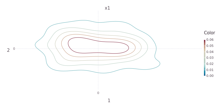
The contour density relates to the distribution of marginal samples as seen with this Gadfly.jl package histogram comparison.
pl1 = drawPoses(fg, to=0);
X0 = getVal(fg, :x0);
pl2 = Gadfly.plot(x=X0[1,:],y=X0[2,:], Geom.hexbin);
plH = hstack(pl1, pl2)
# Gadfly.draw(PNG("/tmp/testH.png",20cm,10cm),plH)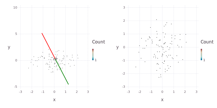
NOTE Red and Green lines represent Port and Starboard direction of Pose2, respectively.
Multiple beliefs can be plotted at the same time, while setting levels=4 rather than the default value:
plX1 = plotKDE(fg, [:x0; :x1], dims=[1;2], levels=4)
# Gadfly.draw(PNG("/tmp/testX1.png",20cm,10cm),plX1)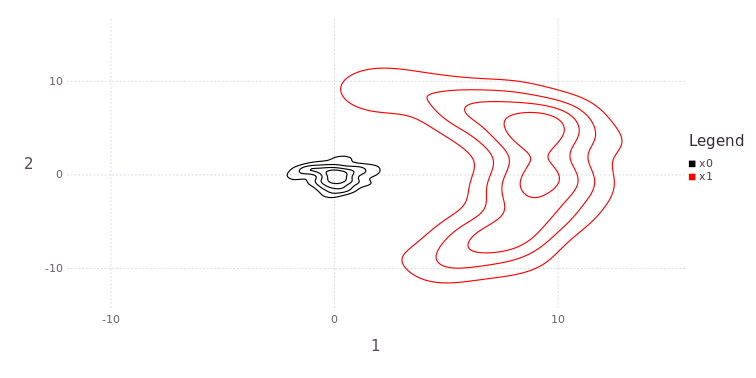
One dimensional (such as Θ) or a stack of all plane projections is also available:
plTh = plotKDE(fg, [:x0; :x1], dims=[3], levels=4)
# Gadfly.draw(PNG("/tmp/testTh.png",20cm,10cm),plTh)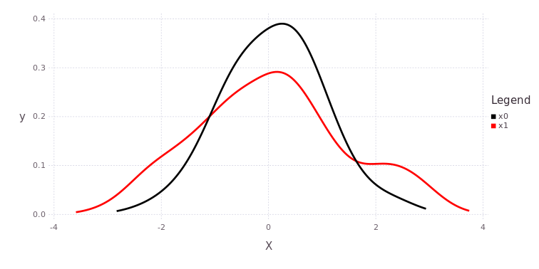
plAll = plotKDE(fg, [:x0; :x1], levels=3)
# Gadfly.draw(PNG("/tmp/testX1.png",20cm,15cm),plAll)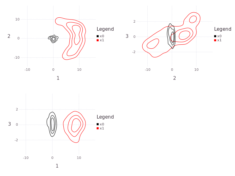
NOTE The functions hstack and vstack is provided through the Gadfly package and allows the user to build a near arbitrary composition of plots.
Please see KernelDensityEstimatePlotting package source for more features.
3D Visualization
Factor graphs of two or three dimensions can be visualized with the 3D visualizations provided by Arena.jl and it's dependencies. The 2D example above and also be visualized in a 3D space with the commands:
vc = startdefaultvisualization() # to load a DrakeVisualizer/Director process instance
visualize(fg, vc, drawlandms=false)
# visualizeallposes!(vc, fg, drawlandms=false)
Here is a basic example of using visualization and multi-core factor graph solving:
addprocs(2)
using Caesar, RoME, TransformUtils, Distributions

# load scene and ROV model (might experience UDP packet loss LCM buffer not set)
sc1 = loadmodel(:scene01); sc1(vc)
rovt = loadmodel(:rov); rovt(vc)

initCov = 0.001*eye(6); [initCov[i,i] = 0.00001 for i in 4:6];
odoCov = 0.0001*eye(6); [odoCov[i,i] = 0.00001 for i in 4:6];
rangecov, bearingcov = 3e-4, 2e-3

# start and add to a factor graph
fg = identitypose6fg(initCov=initCov)
tf = SE3([0.0;0.7;0.0], Euler(pi/4,0.0,0.0) )
addOdoFG!(fg, Pose3Pose3(MvNormal(veeEuler(tf), odoCov) ) )

addLinearArrayConstraint(fg, (4.0, 0.0), :x0, :l1, rangecov=rangecov,bearingcov=bearingcov)
addLinearArrayConstraint(fg, (4.0, 0.0), :x1, :l1, rangecov=rangecov,bearingcov=bearingcov)

solveBatch!(fg)

using Arena

vc = startdefaultvisualization()
visualize(fg, vc, drawlandms=true, densitymeshes=[:l1;:x2])
visualizeDensityMesh!(vc, fg, :l1)
# visualizeallposes!(vc, fg, drawlandms=false)
Previous 3D Viewer (VTK / Director) – no longer required
Previous versions used the much larger VTK based Director available via DrakeVisualizer.jl package. This requires the following preinstalled packages:
sudo apt-get install libvtk5-qt4-dev python-vtk