Multimodal incremental Smoothing and Mapping Algorithm

Work In Progress

Placeholder for details on how the approximate sum-product inference algorithm (mmiSAM) works. Until then, see related literature for more details.

Algorithm combats the so called curse-of-dimensionality on the basis of eight principles outlined in the thesis work "Multimodal and Inertial Sensor Solutions to Navigation-type Factor Graphs".

Joint Probability

mmfgbt

Inference on Bayes/Junction/Elimination Tree

See tree solve video here.

Focussing Computation on Tree

Federated Tree Solution (Multi session/agent)

Tentatively see the multisession page.

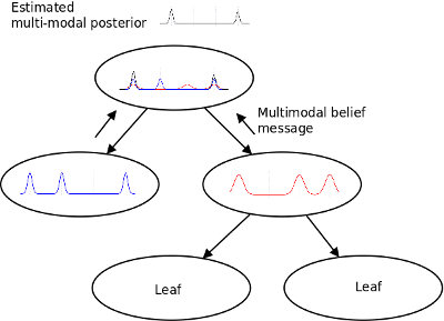
Chapman-Kolmogorov (Belief Propagation / Sum-product)

The main computational effort is to focus compute cycles on dominant modes exhibited by the data, by dropping low likelihood modes (although not indefinitely) and not sacrificing accuracy individual major features.

Clique State Machine

The CSM is used to govern the inference process within a clique. A FunctionalStateMachine.jl implementation is used to allow for initialization / incremental-recycling / fixed-lag solving, and will soon support federated branch solving as well as unidirectional message passing for fixed-lead operations. See the following video for an auto-generated–-using csmAnimate–-concurrent clique solving example.

Sequential Nested Gibbs Method

Current default inference method.

Convolution Approximation (Quasi-Deterministic)

Convolution operations are used to implement the numerical computation of the probabilistic chain rule:

\[P(A, B) = P(A | B)P(B)\]

Proposal distributions are computed by means of (analytical or numerical – i.e. "algebraic") factor which defines a residual function:

\[\delta : S \times \Eta \rightarrow \mathcal{R}\]

where $S \times \Eta$ is the domain such that $\theta_i \in S, \, \eta \sim P(\Eta)$, and $P(\cdot)$ is a probability.

A trust-region, nonlinear gradient decent method is used to enforce the residual function $\delta (\theta_S)$ in a leave-one-out-Gibbs strategy for all the factors and variables in each clique. Each time a factor residual is enforced for another particle along with a sample from the stochastic noise term. Solutions are found either through root finding on "full dimension" equations (source code here):

\[\text{solve}_{\theta_i} ~ s.t. \, 0 = \delta(\theta_{S}; \eta)\]

Or minimization of "low dimension" equations (source code here) that might not have any roots in $\theta_i$:

\[\text{argmin}_{\theta_i} ~ [\delta(\theta_{S}; \eta)]^2\]

Gradient decent methods are obtained from the Julia Package community, namely NLsolve.jl and Optim.jl.

The factor noise term can be any samplable belief (a.k.a. IIF.SamplableBelief), either through algebraic modeling, or (critically) directly from the sensor measurement that is driven by the underlying physics process. Parametric factors (Distributions.jl) or direct physical measurement noise can be used via AliasingScalarSampler or KernelDensityEstimate.

This figure shows an example of the quasi-deterministic convolution of green and red functions to produce the black trace as proposal distribution

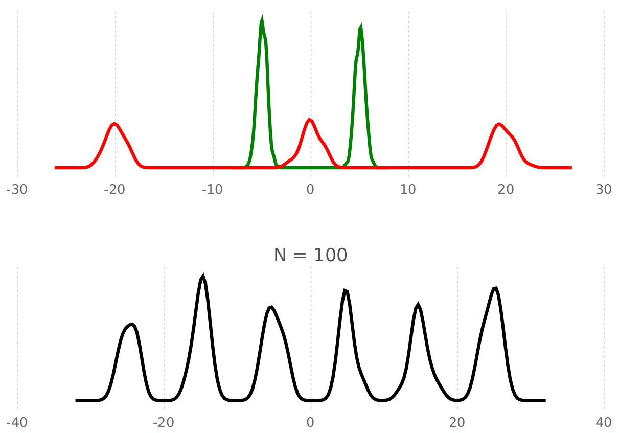
Also see [1.2], Chap. 5, Approximate Convolutions.

Stochastic Product Approx of Infinite Functionals

See mixed-manifold products presented in the literature section.

writing in progress

Mixture Parametric Method

Work In Progress – deferred for progress on full functional methods, but likely to have Gaussian legacy algorithm with mixture model expansion added in the near future.

Full Deterministic Chapman-Kolmogorov Super Product Method

Work in progress, likely to include Kernel Embedding and Homotopy Continuation methods for combining convolution and product operations as a concurrent calculation.