Plotting
Once the graph has been built, 2D plot visualizations are provided by RoMEPlotting.jl and KernelDensityEstimatePlotting.jl. These visualizations tools are readily modifiable to highlight various aspects of mobile platform navigation.
Plotting packages can be installed separately.
Quick Start
A simple usage example:
using RoMEPlotting

drawPoses(fg)
# If you have landmarks, you can instead call
# drawPosesLandms(fg)

# Draw the KDE for x0
plotKDE(fg, :x0)
# Draw the KDE's for x0 and x1
plotKDE(fg, [:x0, :x1])
Hexagonal 2D SLAM example visualization
The major 2D plotting functions between RoMEPlotting.jl:
drawPosesdrawPosesLandmsdrawSubmaps
and KernelDensityEstimatePlotting.jl:
plotKDE/plot(::KernelDensityEstimate)
This simplest example for visualizing a 2D robot trajectory–-such as first running the Hexagonal 2D SLAM example–-
# Assuming some fg<:AbstractDFG has been loaded/constructed
# ...

using RoMEPlotting

# For Juno/Jupyter style use
pl = drawPosesLandms(fg)

# For scripting use-cases you can export the image
Gadfly.draw(PDF("/tmp/test.pdf", 20cm, 10cm),pl)  # or PNG(...)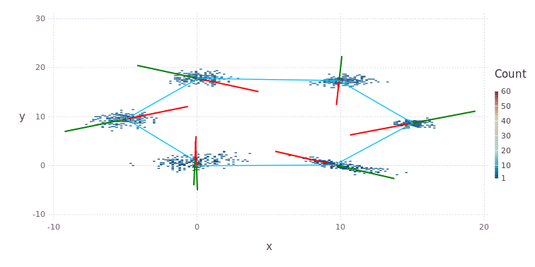
Density Contour Map
KernelDensityEstimatePlotting (as used in RoMEPlotting) provides an interface to visualize belief densities as counter plots. The following basic example shows some of features of the API, where plotKDE(..., dims=[1;2]) implies the marginal over variables (x,y):
using RoME, Distributions
using RoMEPlotting

fg = initfg()
addVariable!(fg, :x0, Pose2)
addFactor!(fg, [:x0], PriorPose2(MvNormal(zeros(3), eye(3))))
addVariable!(fg, :x1, Pose2)
addFactor!(fg, [:x0;:x1], Pose2Pose2(MvNormal([10.0;0;0], eye(3))))

ensureAllInitialized!(fg)

# plot one contour density
plX0 = plotKDE(fg, :x0, dims=[1;2])
# using Gadfly; Gadfly.draw(PNG("/tmp/testX0.png",20cm,10cm),plX0)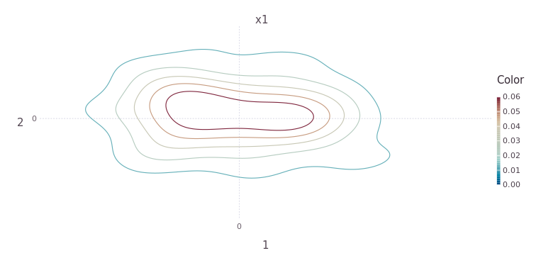
The contour density relates to the distribution of marginal samples as seen with this Gadfly.jl package histogram comparison.
pl1 = drawPoses(fg, to=0);
X0 = getVal(fg, :x0);
pl2 = Gadfly.plot(x=X0[1,:],y=X0[2,:], Geom.hexbin);
plH = hstack(pl1, pl2)
# Gadfly.draw(PNG("/tmp/testH.png",20cm,10cm),plH)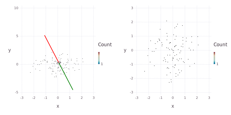
Red and Green lines represent Port and Starboard direction of Pose2, respectively.
Multiple beliefs can be plotted at the same time, while setting levels=4 rather than the default value:
plX1 = plotKDE(fg, [:x0; :x1], dims=[1;2], levels=4)
# Gadfly.draw(PNG("/tmp/testX1.png",20cm,10cm),plX1)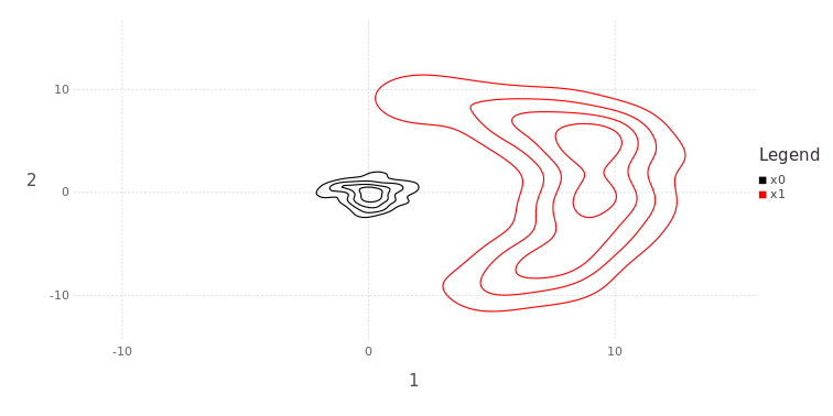
One dimensional (such as Θ) or a stack of all plane projections is also available:
plTh = plotKDE(fg, [:x0; :x1], dims=[3], levels=4)
# Gadfly.draw(PNG("/tmp/testTh.png",20cm,10cm),plTh)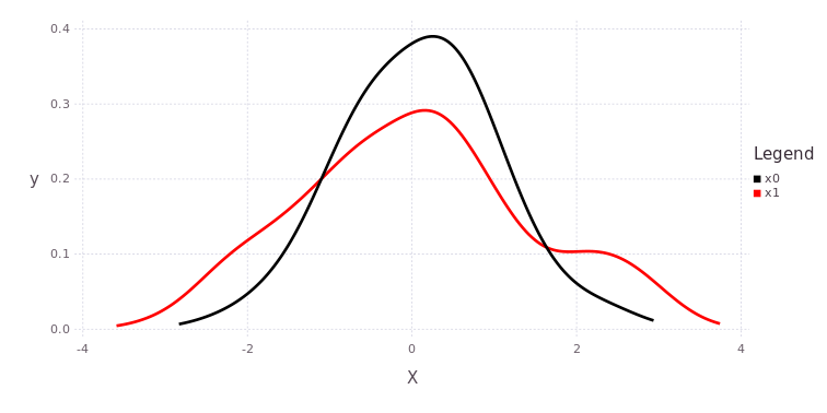
plAll = plotKDE(fg, [:x0; :x1], levels=3)
# Gadfly.draw(PNG("/tmp/testX1.png",20cm,15cm),plAll)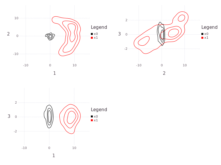
The functions hstack and vstack is provided through the Gadfly package and allows the user to build a near arbitrary composition of plots.
Please see KernelDensityEstimatePlotting package source for more features.
Interactive Gadfly.jl Plots
See the following two discussions on Interactive 2D plots: