Tutorial
This tutorial assumes you have already installed Julia and TORA.jl. See Installation.
Setup
We are going to use TORA.jl as well as other packages to visualize and handle rigid-body mechanisms.
using TORA
using MeshCat
using RigidBodyDynamics
Try to call TORA.greet(). It should simply print "Hello World!"
TORA.greet()Hello World!
Next, we want to create a 3D viewer using MeshCat.jl
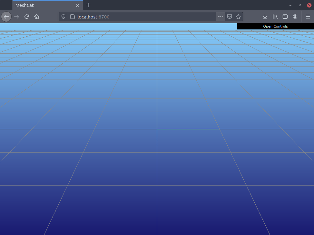
vis = Visualizer()Let's open the visualizer (in a separate browser tab)
open(vis)It should look like this:
Loading a Robot
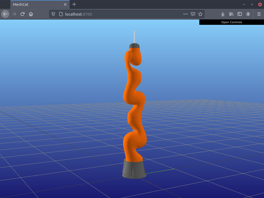
After starting the viewer, we are now ready to load a robot. Let's load a KUKA LBR iiwa 14 with
robot = TORA.create_robot_kuka_iiwa_14(vis)To load a different robot, check the Adding a New Robot page of the documentation.
Afterwards, you should be able to see the robot in the viewer:
Creating a Problem
Having loaded the robot, we are now ready to define the task we want to solve.
TORA.jl uses a Direct Transcription[1] approach to optimize trajectories. This technique splits the trajectory into $N$ equally-spaced[2] segments
where $t_I$ and $t_F$ are the start and final instants, respectively. This division results in $M = N + 1$ discrete mesh points (a.k.a. knots), for each of which TORA.jl discretizes the states of the system, as well as the control inputs.
To create a new problem, we use the TORA.Problem constructor, which takes three arguments:
- a
TORA.Robot, - the number of knots we wish to use for representing the trajectory, and
- the time step duration between each pair of consecutive knots.
Suppose we want to optimize a motion with a total duration of 2 seconds, and that we want to calculate the control inputs to the system at a frequency of 150 Hz.
const duration = 2.0  # in seconds
const hz = 150
In that case, the time step duration would be
dt = 1/1500.006666666666666667
and the total number of knots would be given by
hz * duration + 1301.0
Therefore, we create the problem by running
problem = TORA.Problem(robot, 301, 1/150)We can use TORA.show_problem_info to print a summary of relevant information of a TORA.Problem.
TORA.show_problem_info(problem)Motion duration ...................................... 2.0 seconds Number of knots with constrained joint positions ..... 0 Number of knots with constrained joint velocities .... 0 Number of knots with constrained joint torques ....... 0 Number of knots with constrained ee position ......... 0
The summary above shows that the total duration of the motion is 2.0 seconds, just like we wanted.
The summary also shows that there are no constraints defined yet, as we have just now created the problem.
Defining Constraints
The decision variables of the optimization problem at every knot are:
- joint positions,
- joint velocities, and
- joint torques.[3]
Bounds of the Decision Variables
The bounds of the decision variables need not be defined. They are automatically inferred from the URDF model.
Fixing Values of the Decision Variables
It is possible to fix the values of specific decision variables with:
Suppose we want to enforce zero joint velocities both at the very start of the motion and at the very end of the motion. We can specify such constraints with
# Constrain initial and final joint velocities to zero
TORA.fix_joint_velocities!(problem, robot, 1, zeros(robot.n_v))
TORA.fix_joint_velocities!(problem, robot, problem.num_knots, zeros(robot.n_v))
Let's have a look at the problem summary output again:
TORA.show_problem_info(problem)Motion duration ...................................... 2.0 seconds Number of knots with constrained joint positions ..... 0 Number of knots with constrained joint velocities .... 2 Number of knots with constrained joint torques ....... 0 Number of knots with constrained ee position ......... 0
The output confirms that there are now two knots for which we have fixed specific joint velocities.
End-effector Constraints
TORA.constrain_ee_position! allows us to enforce specific positions for the end-effector of the robot.
If we want the end-effector of the robot to be located at $[0.5, 0.2, 0.3]$ in knot $k = 33$ we would write
TORA.constrain_ee_position!(problem, 33, [0.5, 0.2, 0.3])But let's do something more interesting for this tutorial... Let's define a problem where the robot must trace a circular path. For that, we just need to call TORA.constrain_ee_position! multiple times with the right combination of knot and position such that we describe a circle.
let CubicTimeScaling(Tf::Number, t::Number) = 3(t / Tf)^2 - 2(t / Tf)^3
    for k = 1:2:problem.num_knots  # For every other knot
        θ = CubicTimeScaling(problem.num_knots - 1, k - 1) * 2π
        pos = [0.5, 0.2 * cos(θ), 0.8 + 0.2 * sin(θ)]
        TORA.constrain_ee_position!(problem, k, pos)
    end
end
In the snippet above, CubicTimeScaling is a helper function (a cubic polynomial). It allows us to specify a path for the end-effector that accelerates at first, and decelerates near the end. This is a better alternative to tracing the path with constant velocity.
The for loop inside the let block samples every other knot of the trajectory, and computes the position pos of the end-effector at that knot using the angle $\theta$.
Let's print the problem summary once again:
TORA.show_problem_info(problem)Motion duration ...................................... 2.0 seconds Number of knots with constrained joint positions ..... 0 Number of knots with constrained joint velocities .... 2 Number of knots with constrained joint torques ....... 0 Number of knots with constrained ee position ......... 151
The output correctly shows that we now have end-effector position constraints in 151 knots.
Providing an Initial Guess
Trajectory Optimization problems can be very challenging to solve. As such, providing a good initial guess (starting point) for the trajectory helps solvers significantly.
For our circle-tracing task, we are going to define a very simple (but reasonably good) initial guess: a static configuration, zero velocities, and zero torques.
First, let's define the static configuration:
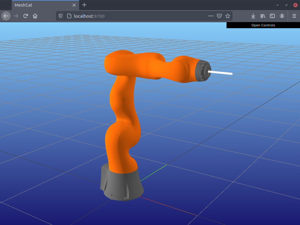
initial_q = [0, 0, 0, -π/2, 0, 0, 0]We can visualize this configuration by running
zero!(robot.state)
set_configuration!(robot.state, initial_q)
set_configuration!(robot.mvis, configuration(robot.state))
This will update the configuration of the robot in the viewer:
We can now define the initial guess for the joint positions with that fixed configuration, repeated for every knot:
initial_qs = repeat(initial_q, 1, problem.num_knots)7×301 Array{Float64,2}:
0.0 0.0 0.0 0.0 … 0.0 0.0 0.0 0.0
0.0 0.0 0.0 0.0 0.0 0.0 0.0 0.0
0.0 0.0 0.0 0.0 0.0 0.0 0.0 0.0
-1.5708 -1.5708 -1.5708 -1.5708 -1.5708 -1.5708 -1.5708 -1.5708
0.0 0.0 0.0 0.0 0.0 0.0 0.0 0.0
0.0 0.0 0.0 0.0 … 0.0 0.0 0.0 0.0
0.0 0.0 0.0 0.0 0.0 0.0 0.0 0.0For the joint velocities we are going to start with zeroes repeated for every knot:
initial_vs = zeros(robot.n_v, problem.num_knots)7×301 Array{Float64,2}:
0.0 0.0 0.0 0.0 0.0 0.0 0.0 0.0 … 0.0 0.0 0.0 0.0 0.0 0.0 0.0
0.0 0.0 0.0 0.0 0.0 0.0 0.0 0.0 0.0 0.0 0.0 0.0 0.0 0.0 0.0
0.0 0.0 0.0 0.0 0.0 0.0 0.0 0.0 0.0 0.0 0.0 0.0 0.0 0.0 0.0
0.0 0.0 0.0 0.0 0.0 0.0 0.0 0.0 0.0 0.0 0.0 0.0 0.0 0.0 0.0
0.0 0.0 0.0 0.0 0.0 0.0 0.0 0.0 0.0 0.0 0.0 0.0 0.0 0.0 0.0
0.0 0.0 0.0 0.0 0.0 0.0 0.0 0.0 … 0.0 0.0 0.0 0.0 0.0 0.0 0.0
0.0 0.0 0.0 0.0 0.0 0.0 0.0 0.0 0.0 0.0 0.0 0.0 0.0 0.0 0.0And the same for the joint torques:
initial_τs = zeros(robot.n_τ, problem.num_knots)7×301 Array{Float64,2}:
0.0 0.0 0.0 0.0 0.0 0.0 0.0 0.0 … 0.0 0.0 0.0 0.0 0.0 0.0 0.0
0.0 0.0 0.0 0.0 0.0 0.0 0.0 0.0 0.0 0.0 0.0 0.0 0.0 0.0 0.0
0.0 0.0 0.0 0.0 0.0 0.0 0.0 0.0 0.0 0.0 0.0 0.0 0.0 0.0 0.0
0.0 0.0 0.0 0.0 0.0 0.0 0.0 0.0 0.0 0.0 0.0 0.0 0.0 0.0 0.0
0.0 0.0 0.0 0.0 0.0 0.0 0.0 0.0 0.0 0.0 0.0 0.0 0.0 0.0 0.0
0.0 0.0 0.0 0.0 0.0 0.0 0.0 0.0 … 0.0 0.0 0.0 0.0 0.0 0.0 0.0
0.0 0.0 0.0 0.0 0.0 0.0 0.0 0.0 0.0 0.0 0.0 0.0 0.0 0.0 0.0We can concatenate these matrices into a single one:
initial_guess = [initial_qs; initial_vs; initial_τs]21×301 Array{Float64,2}:
0.0 0.0 0.0 0.0 … 0.0 0.0 0.0 0.0
0.0 0.0 0.0 0.0 0.0 0.0 0.0 0.0
0.0 0.0 0.0 0.0 0.0 0.0 0.0 0.0
-1.5708 -1.5708 -1.5708 -1.5708 -1.5708 -1.5708 -1.5708 -1.5708
0.0 0.0 0.0 0.0 0.0 0.0 0.0 0.0
0.0 0.0 0.0 0.0 … 0.0 0.0 0.0 0.0
0.0 0.0 0.0 0.0 0.0 0.0 0.0 0.0
0.0 0.0 0.0 0.0 0.0 0.0 0.0 0.0
0.0 0.0 0.0 0.0 0.0 0.0 0.0 0.0
0.0 0.0 0.0 0.0 0.0 0.0 0.0 0.0
⋮ ⋱ ⋮
0.0 0.0 0.0 0.0 0.0 0.0 0.0 0.0
0.0 0.0 0.0 0.0 0.0 0.0 0.0 0.0
0.0 0.0 0.0 0.0 0.0 0.0 0.0 0.0
0.0 0.0 0.0 0.0 … 0.0 0.0 0.0 0.0
0.0 0.0 0.0 0.0 0.0 0.0 0.0 0.0
0.0 0.0 0.0 0.0 0.0 0.0 0.0 0.0
0.0 0.0 0.0 0.0 0.0 0.0 0.0 0.0
0.0 0.0 0.0 0.0 0.0 0.0 0.0 0.0
0.0 0.0 0.0 0.0 … 0.0 0.0 0.0 0.0Notice that the dimensions are 21×301, i.e., the dimension of each knot ($\mathbb{R}^{21}$) times the 301 knots.
We can flatten this matrix into a vector with
initial_guess = vec(initial_guess)Julia follows a column-major convention. See Access arrays in memory order, along columns.
As a very last step, we just need to truncate the last few values that correspond to the control inputs at the last knot. The last knot represents the end of the motion, so we only represent the robot state.
initial_guess = initial_guess[1:end - robot.n_τ]Solving the Problem
Once we are happy with the problem definition, we just need to call solve and the optimization will start.
cpu_time, x, solver_log = TORA.solve_with_ipopt(problem, robot, initial_guess=initial_guess)
******************************************************************************
This program contains Ipopt, a library for large-scale nonlinear optimization.
 Ipopt is released as open source code under the Eclipse Public License (EPL).
         For more information visit http://projects.coin-or.org/Ipopt
******************************************************************************

This is Ipopt version 3.13.2, running with linear solver mumps.
NOTE: Other linear solvers might be more efficient (see Ipopt documentation).

Number of nonzeros in equality constraint Jacobian...:    90962
Number of nonzeros in inequality constraint Jacobian.:        0
Number of nonzeros in Lagrangian Hessian.............:        0

Total number of variables............................:     6300
                     variables with only lower bounds:        0
                variables with lower and upper bounds:     6300
                     variables with only upper bounds:        0
Total number of equality constraints.................:     4653
Total number of inequality constraints...............:        0
        inequality constraints with only lower bounds:        0
   inequality constraints with lower and upper bounds:        0
        inequality constraints with only upper bounds:        0

iter    objective    inf_pr   inf_du lg(mu)  ||d||  lg(rg) alpha_du alpha_pr  ls
   0  0.0000000e+00 2.22e-01 0.00e+00   0.0 0.00e+00    -  0.00e+00 0.00e+00   0
   1  0.0000000e+00 2.18e-01 2.01e+02   0.5 1.54e+01    -  9.51e-01 1.00e+00h  1
   2  0.0000000e+00 1.58e-01 9.21e+02   0.4 7.12e+00    -  1.00e+00 1.00e+00h  1
   3  0.0000000e+00 3.32e-02 7.63e+03  -0.3 5.69e+00    -  1.00e+00 1.00e+00h  1
   4  0.0000000e+00 3.21e-03 2.13e+02  -1.0 1.89e+00    -  1.00e+00 1.00e+00h  1
   5  0.0000000e+00 2.09e-05 4.05e-01  -3.1 5.51e-02    -  9.87e-01 1.00e+00h  1
   6  0.0000000e+00 3.98e-07 7.84e-02  -4.6 9.72e-03    -  1.00e+00 1.00e+00h  1
   7  0.0000000e+00 1.25e-08 1.15e-03  -6.4 1.80e-03  -4.0 1.00e+00 1.00e+00h  1
   8  0.0000000e+00 1.63e-11 6.24e-09  -8.5 5.88e-05  -4.5 1.00e+00 1.00e+00h  1

Number of Iterations....: 8

                                   (scaled)                 (unscaled)
Objective...............:   0.0000000000000000e+00    0.0000000000000000e+00
Dual infeasibility......:   6.2393222275142777e-09    6.2393222275142777e-09
Constraint violation....:   1.6266155089539325e-11    1.6266155089539325e-11
Complementarity.........:   2.9079800276678474e-09    2.9079800276678474e-09
Overall NLP error.......:   6.2393222275142777e-09    6.2393222275142777e-09


Number of objective function evaluations             = 9
Number of objective gradient evaluations             = 9
Number of equality constraint evaluations            = 9
Number of inequality constraint evaluations          = 0
Number of equality constraint Jacobian evaluations   = 9
Number of inequality constraint Jacobian evaluations = 0
Number of Lagrangian Hessian evaluations             = 0
Total CPU secs in IPOPT (w/o function evaluations)   =      0.726
Total CPU secs in NLP function evaluations           =      0.328

EXIT: Optimal Solution Found.There exist additional parameters that you can pass to TORA.solve_with_*. See Solver Interfaces.
Showing the Results
When the optimization finishes, we can playback the trajectory on the robot shown in the viewer.
TORA.play_trajectory(vis, problem, robot, x)You should be able to see this:
We can also plot the positions, velocities, and torques of the obtained trajectory:
TORA.plot_results(problem, robot, x)Lastly, we can plot the TORA.SolverLog (returned by the solve function) to study the evolution of the feasibility error and of the objective function value (if one has been defined) per iteration.
TORA.plot_log(solver_log)That concludes this tutorial. Congratulations! And thank you for sticking around this far.

- 1Betts, John T. Practical Methods for Optimal Control and Estimation Using Nonlinear Programming. SIAM, 2010.
- 2Direct Transcription does not necessarily require equally-spaced segments.
- 3An exception to this is the last knot, which only discretizes joint positions and joint velocities.