Plotting 2D
Once the graph has been built, 2D plot visualizations are provided by RoMEPlotting.jl and KernelDensityEstimatePlotting.jl. These visualizations tools are readily modifiable to highlight various aspects of mobile platform navigation.
Plotting packages can be installed separately.
The major 2D plotting functions between RoMEPlotting.jl and KernelDensityEstimatePlotting.jl:
plotSLAM2D,plotSLAM2DPoses,plotSLAM2DLandmarks,plotPose,plotBelief- LEGACY
plotKDE plotLocalProduct,PDF,PNG,SVG,hstack,vstack.
Example Plot SLAM 2D
This simplest example for visualizing a 2D robot trajectory–-such as first running the Hexagonal 2D SLAM example–-
Assuming some fg<:AbstractDFG has been loaded/constructed:
# load the plotting functionality
using RoME, RoMEPlotting
# generate some factor graph with numerical values
fg = generateGraph_Hexagonal()
solveTree!(fg)
# or fg = loadDFG("somepath")
# slam2D plot
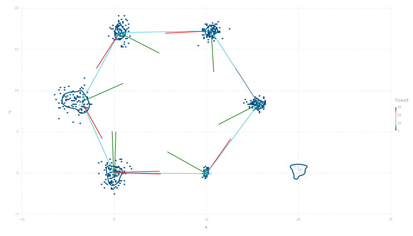
pl = plotSLAM2D(fg, drawhist=true, drawPoints=false)
RoMEPlotting.plotSLAM2D — FunctionplotSLAM2D(
fgl;
solveKey,
from,
to,
minnei,
meanmax,
posesPPE,
landmsPPE,
recalcPPEs,
lbls,
scale,
x_off,
y_off,
drawTriads,
dyadScale,
levels,
drawhist,
MM,
xmin,
xmax,
ymin,
ymax,
showmm,
window,
point_size,
line_width,
regexLandmark,
regexPoses,
variableList,
manualColor,
drawPoints,
pointsColor,
drawContour,
drawEllipse,
ellipseColor,
title,
aspect_ratio
)
2D plot of both poses and landmarks contained in factor graph. Assuming poses and landmarks are labeled :x1, :x2, ... and :l0, :l1, ..., respectively. The range of numbers to include can be controlled with from and to along with other keyword functionality for manipulating the plot.
Notes
- Assumes
:l1,:l2, ... for landmarks – - Can increase default Gadfly plot size (for JSSVG in browser):
Gadfly.set_default_plot_size(35cm,20cm). - Enable or disable features such as the covariance ellipse with keyword
drawEllipse=true.
DevNotes
- TODO update to use e.g.
tags=[:LANDMARK], - TODO fix
drawHist, - TODO deprecate,
showmm,spscale.
Examples:
fg = generateGraph_Hexagonal()
plotSLAM2D(fg)
plotSLAM2D(fg, drawPoints=false)
plotSLAM2D(fg, contour=false, drawEllipse=true)
plotSLAM2D(fg, contour=false, title="SLAM result 1")

# or load a factor graph
fg_ = loadDFG("somewhere.tar.gz")
plotSLAM2D(fg_)
Related
Plot Covariance Ellipse and Points
While the Caesar.jl framework is focussed on non-Gaussian inference, it is frequently desirable to relate the results to a more familiar covariance ellipse, and native support for this exists:
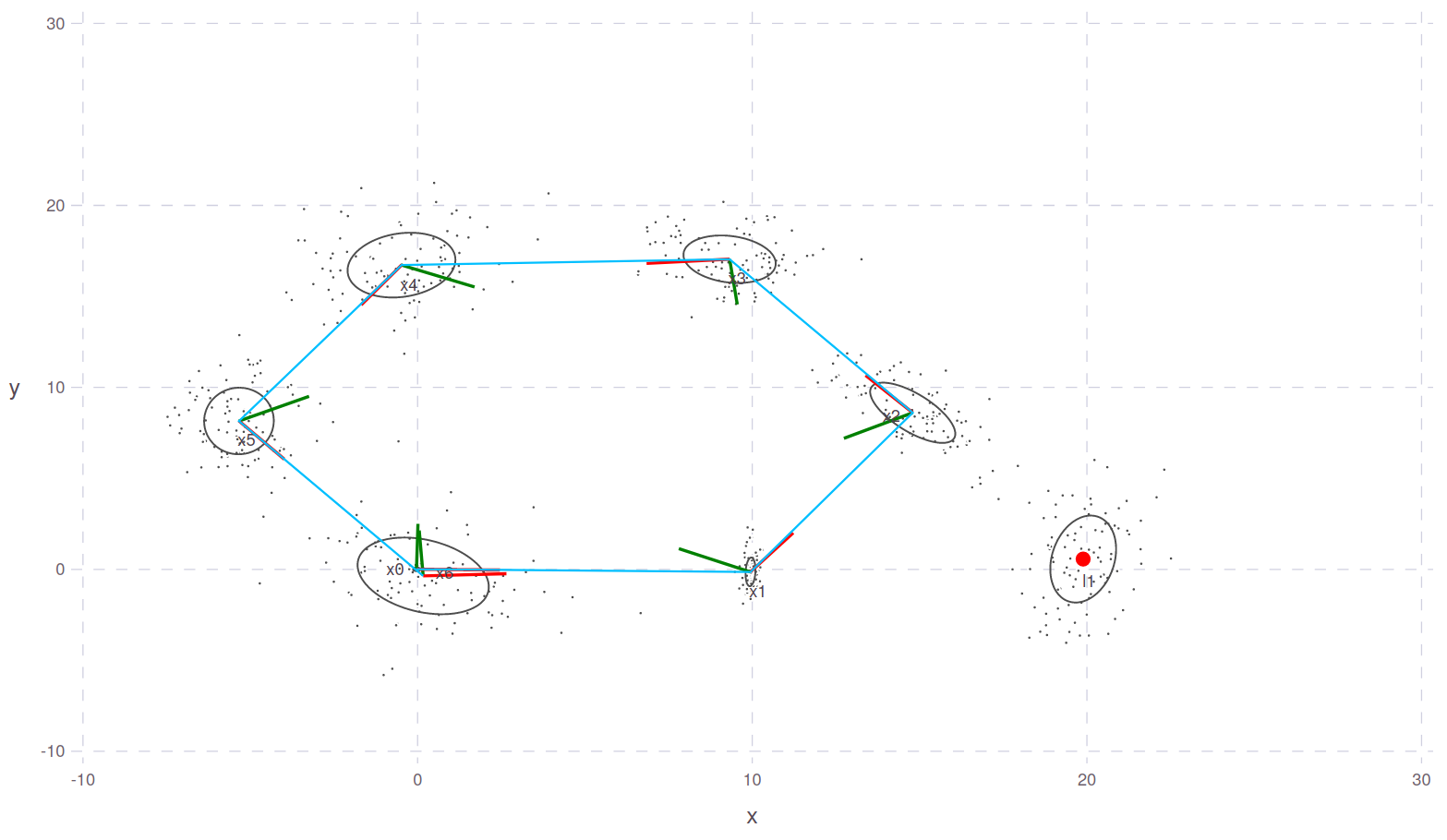
plotSLAM2D(fg, drawContour=false, drawEllipse=true, drawPoints=true)
Plot Poses or Landmarks
Lower down utility functions are used to plot poses and landmarks separately before joining the Gadfly layers.
RoMEPlotting.plotSLAM2DPoses — FunctionplotSLAM2DPoses(
fg;
solveKey,
regexPoses,
from,
to,
variableList,
meanmax,
ppe,
recalcPPEs,
lbls,
scale,
x_off,
y_off,
drawhist,
spscale,
dyadScale,
drawTriads,
drawContour,
levels,
contour,
line_width,
drawPoints,
pointsColor,
drawEllipse,
ellipseColor,
manualColor
)
2D plot of all poses, assuming poses are labeled from `::Symbol type :x0, :x1, ..., :xn. Use to and from to limit the range of numbers n to be drawn. The underlying histogram can be enabled or disabled, and the size of maximum-point belief estimate cursors can be controlled with spscale.
Future:
- Relax to user defined pose labeling scheme, for example
:p1, :p2, ...
RoMEPlotting.plotSLAM2DLandmarks — FunctionplotSLAM2DLandmarks(
fg;
solveKey,
regexLandmark,
from,
to,
minnei,
variableList,
meanmax,
ppe,
recalcPPEs,
lbls,
showmm,
scale,
x_off,
y_off,
drawhist,
drawContour,
levels,
contour,
manualColor,
c,
MM,
point_size,
drawPoints,
pointsColor,
drawEllipse,
ellipseColor,
resampleGaussianFit
)
2D plot of landmarks, assuming :l1, :l2, ... :ln. Use from and to to control the range of landmarks n to include.
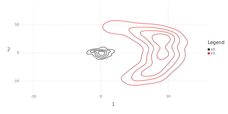
Plot Belief Density Contour
KernelDensityEstimatePlotting (as used in RoMEPlotting) provides an interface to visualize belief densities as counter plots. Something basic might be to just show all plane pairs of this variable marginal belief:
# Draw the KDE for x0
plotBelief(fg, :x0)
Plotting the marginal density over say variables (x,y) in a Pose2 would be:
plotBelief(fg, :x1, dims=[1;2])The following example better shows some of features (via Gadfly.jl):
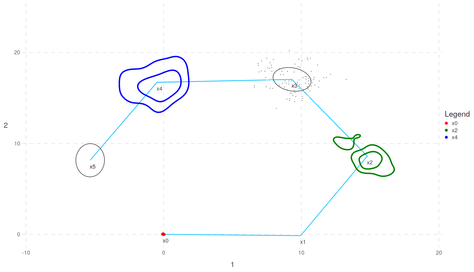
# Draw the (x,y) marginal estimated belief contour for :x0, :x2, and Lx4
pl = plotBelief(fg, [:x0; :x2; :x4], c=["red";"green";"blue"], levels=2, dims=[1;2])

# add a few fun layers
pl3 = plotSLAM2DPoses(fg, regexPoses=r"x\d", from=3, to=3, drawContour=false, drawEllipse=true)
pl5 = plotSLAM2DPoses(fg, regexPoses=r"x\d", from=5, to=5, drawContour=false, drawEllipse=true, drawPoints=false)
pl_ = plotSLAM2DPoses(fg, drawContour=false, drawPoints=false, dyadScale=0.001, to=5)
union!(pl.layers, pl3.layers)
union!(pl.layers, pl5.layers)
union!(pl.layers, pl_.layers)

# change the plotting coordinates
pl.coord = Coord.Cartesian(xmin=-10,xmax=20, ymin=-1, ymax=25)

# save the plot to SVG and giving dedicated (although optional) sizing
pl |> SVG("/tmp/test.svg", 25cm, 15cm)

# also display the plot live
pl
See function documentation for more details on API features
RoMEPlotting.plotBelief — FunctionplotBelief(
fgl,
sym;
solveKey,
dims,
title,
levels,
fill,
layers,
c,
overlay
)
A peneric KDE plotting function that allows marginals of higher dimensional beliefs and various keyword options.
Example for Position2:
p = manikde!(Position2, [randn(2) for _ in 1:100])
q = manikde!(Position2, [randn(2).+[5;0] for _ in 1:100])

plotBelief(p)
plotBelief(p, dims=[1;2], levels=3)
plotBelief(p, dims=[1])

plotBelief([p;q])
plotBelief([p;q], dims=[1;2], levels=3)
plotBelief([p;q], dims=[1])
Example for Pose2:
# TODOSave Plot to Image
VSCode/Juno can set plot to be opened in a browser tab instead. For scripting use-cases you can also export the image:
using Gadfly
# can change the default plot size
# Gadfly.set_default_plot_size(35cm, 30cm)

pl |> PDF("/tmp/test.pdf", 20cm, 10cm)  # or PNG, SVG
Save Plot Object To File
It is also possible to store the whole plot container to file using JLD2.jl:
JLD2.@save "/tmp/myplot.jld2" pl

# and loading elsewhere
JLD2.@load "/tmp/myplot.jld2" pl
Interactive Plots, Zoom, Pan (Gadfly.jl)
See the following two discussions on Interactive 2D plots:
Red and Green dyad lines represent the visualization-only assumption of X-forward and Y-left direction of Pose2. The inference and manifold libraries surrounding Caesar.jl are agnostic to any particular choice of reference frame alignment, such as north east down (NED) or forward left up (common in mobile robotics).
Also see Gadfly.jl notes about hstack and vstack to combine plots side by side or vertically.
Plot Pose Individually
It is also possible to plot the belief density of a Pose2 on-manifold:
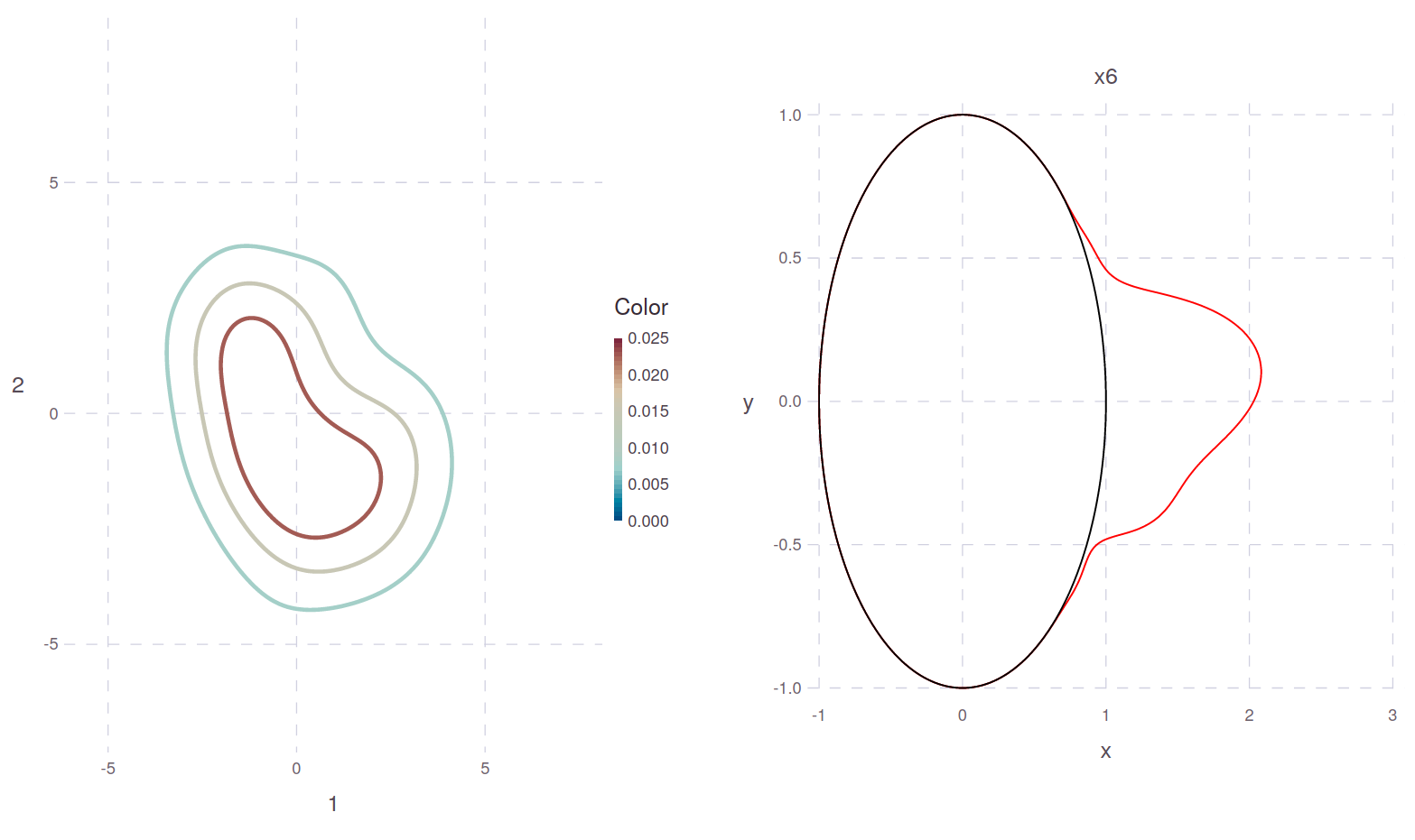
plotPose(fg, :x6)
RoMEPlotting.plotPose — FunctionplotPose(, pp; ...)
plotPose(
,
pp,
title;
levels,
c,
legend,
axis,
scale,
overlay,
hdl
)
Plot pose belief as contour information on visually sensible manifolds.
Example:
fg = generateGraph_ZeroPose()
initAll!(fg);
plotPose(fg, :x0)
Related
plotSLAM2D, plotSLAM2DPoses, plotBelief, plotKDECircular
plotPose(
    fgl,
    syms;
    solveKey,
    levels,
    c,
    axis,
    scale,
    show,
    filepath,
    app,
    hdl
)
Example: pl = plotPose(fg, [:x1; :x2; :x3])
Debug With Local Graph Product Plot
One useful function is to check that data in the factor graph makes sense. While the full inference algorithm uses a Bayes (Junction) tree to assemble marginal belief estimates in an efficient manner, it is often useful for a straight forward graph based sanity check. The plotLocalProduct projects through approxConvBelief each of the factors connected to the target variable and plots the result. This example looks at the loop-closure point around :x0, which is also pinned down by the only prior in the canonical Hexagonal factor graph.
@show ls(fg, :x0);
# ls(fg, :x0) = [:x0f1, :x0x1f1, :x0l1f1]

pl = plotLocalProduct(fg, :x0, dims=[1;2], levels=1)
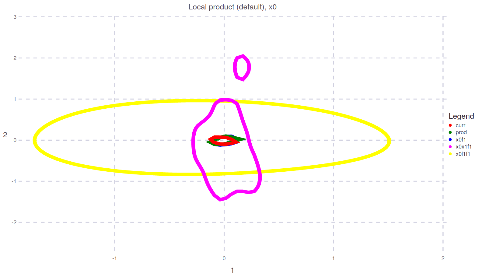
While perhaps a little cluttered to read at first, this figure shows that a new calculation local to only the factor graph prod in greem matches well with the existing value curr in red in the fg from the earlier solveTree! call. These values are close to the prior prediction :x0f1 in blue (fairly trivial case), while the odometry :x0x1f1 and landmark sighting projection :x0l1f1 are also well in agreement.
RoMEPlotting.plotLocalProduct — FunctionplotLocalProduct(
fgl,
lbl;
solveKey,
N,
dims,
levels,
show,
dirpath,
mimetype,
sidelength,
title,
xmin,
xmax,
ymin,
ymax
)
Plot the proposal belief from neighboring factors to lbl in the factor graph (ignoring Bayes tree representation), and show with new product approximation for reference.
DevNotes
- TODO, standardize around ::MIME="image/svg", see JuliaRobotics/DistributedFactorGraphs.jl#640
plotLocalProduct(fgl, lbl; N, dims)
Plot the proposal belief from neighboring factors to lbl in the factor graph (ignoring Bayes tree representation), and show with new product approximation for reference. String version is obsolete and will be deprecated.
More Detail About Density Plotting
Multiple beliefs can be plotted at the same time, while setting levels=4 rather than the default value:
plX1 = plotBelief(fg, [:x0; :x1], dims=[1;2], levels=4)

# plX1 |> PNG("/tmp/testX1.png")
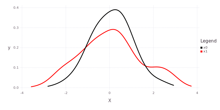
One dimensional (such as Θ) or a stack of all plane projections is also available:
plTh = plotBelief(fg, [:x0; :x1], dims=[3], levels=4)

# plTh |> PNG("/tmp/testTh.png")
plAll = plotBelief(fg, [:x0; :x1], levels=3)
# plAll |> PNG("/tmp/testX1.png",20cm,15cm)
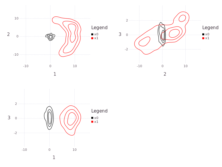
The functions hstack and vstack is provided through the Gadfly package and allows the user to build a near arbitrary composition of plots.
Please see KernelDensityEstimatePlotting package source for more features.