Build your own (Bayes) Filter
Correspondence with Kalman Filtering?
A frequent discussion point is the correspondence between Kalman/particle/log-flow filtering strategies and factor graph formulations. This section aims to shed light on the relationship, and to show that factor graph interpretations are a powerful generalization of existing filtering techniques. The discussion follows a build-your-own-filter style and combines the Approximate Convolution and Multiplying Densities pages as the required prediction and update cycle steps, respectively. Using the steps described here, the user will be able to build fully-functional–-i.e. non-Gaussian–-(Bayes) filters.
A simple 1D predict correct Bayesian filtering example (using underlying convolution and product operations of the mmisam algorithm) can be used as a rough template to familiarize yourself on the correspondence between filters and newer graph-based operations.
This page tries to highlight some of the reasons why using a factor graph approach (w/ Bayes/junction tree inference) in a incremental/fixed-lag/federated sense–-e.g. simultaneous localization and mapping (SLAM) approach–-has merit. The described steps form part of the core operations used by the multimodal incremental smoothing and mapping (mmisam) algorithm.
Further topics on factor graph (and Bayes/junction tree) inference formulation, including how out-marginalization works is discussed separately as part of the Bayes tree description page. It is also worth reiterating the section on why do we even care about non-Gaussian signal processing.
Coming soon, the steps described on this page will be fully accessible via multi-language interfaces (middleware) – some of these interfaces already exist.
Causality and Markov Assumption
WIP: Causal connection explanation: How is the graph based method the same as Kalman filtering variants (UKF, EKF), including Bayesian filtering (PF, etc.), and the Hidden Markov Model (HMM) methodology.
Furthermore, see below for connection to EKF-SLAM too.
Joint Probability and Chapman-Kolmogorov
WIP; The high level task is to "invert" measurements Z give the state of the world Theta
Maximum Likelihood vs. Message Passing
WIP; This dicussion will lead towards Bayesian Networks (Pearl) and Bayes Trees (Kaess et al., Fourie et al.).
The Target Tracking Problem (Conventional Filtering)
Consider a common example, two dimensional target tracking, where a projectile transits over a tracking station using various sensing technologies [Zarchan 2013]. Position and velocity estimates of the target
Prediction Step using a Factor Graph
Assume a constant velocity model from which the estimate will be updated through the measurement model described in the next section. A constant velocity model is taken as (cartesian)
\[\frac{dx}{dt} = 0 + \eta_x\\ \frac{dy}{dt} = 0 + \eta_y\]
or polar coordinates
\[\frac{d\rho}{dt} = 0 + \eta_{\rho}\\ \frac{d\theta}{dt} = 0 + \eta_{\theta}.\]
In this example, noise is introduced as an affine slack variable \eta, but could be added as any part of the process model:
\[\eta_j \sim p(...)\]
where p is any allowable noise probability density/distribution model – discussed more in the next section.
After integration (assume zeroth order) the associated residual function can be constructed:
\[\delta_i (\theta_{k}, \theta_{k-1}, \frac{d \theta_k}{dt}; \Delta t) = \theta_{k} - (\theta_{k-1} + \frac{d \theta_k}{dt} \Delta t)\]
Filter prediction steps are synonymous with a binary factor (conditional likelihood) between two variables where a prior estimate from one variable is projected (by means of a convolution) to the next variable. The convolutional principle page describes a more detailed example on how a convolution can be computed.
Measurement Step using a Factor Graph
The measurement update is a product operation of infinite functional objects (probability densities)
\[p(X_k | X_{k-1}, Z_a, Z_b) \approx p(X_k | X_{k-1}, Z_a) \times p(X_k | Z_b),\]
where Z_. represents conditional information for two beliefs on the same variable. The product of the two functional estimates (beliefs) are multiplied by a stochastic algorithm described in more detail on the multiplying functions page.
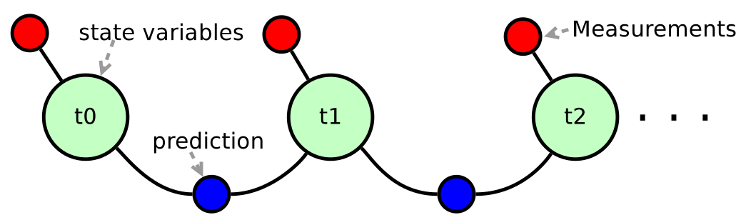
Direct state observations can be added to the factor graph as prior factors directly on the variables. An illustration of both predictions (binary likelihood process model) and direct observations (measurements) is presented:
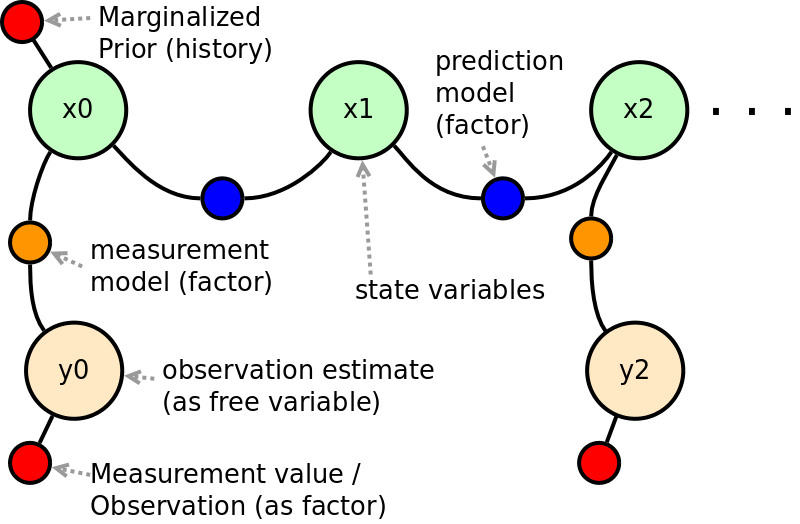
Alternatively, indirect measurements of the state variables are should be modeled with the most sensible function
\[y = h(\theta, \eta)\\ \delta_j(\theta_j, \eta_j) = \ominus h_j(\theta_j, \eta_j) \oplus y_j,\]
which approximates the underlying (on-manifold) stochastics and physics of the process at hand. The measurement models can be used to project belief through a measurement function, and should be recognized as a standard representation for a Hidden Markov Model (HMM):
Beyond Filtering
Consider a multi-sensory system along with data transmission delays, variable sampling rates, etc.; when designing a filtering system to track one or multiple targets, it quickly becomes difficult to augment state vectors with the required state and measurement histories. In contrast, the factor graph as a language allows for heterogeneous data streams to be combined in a common inference framework, and is discussed further in the building distributed factor graphs section.
Factor graphs are constructed along with the evolution of time which allows the mmisam inference algorithm to resolve variable marginal estimates both forward and backwards in time. Conventional filtering only allows for forward-backward "smoothing" as two separate processes. When inferring over a factor graph, all variables and factors are considered simultaneously according the topological connectivity irrespective of when and where which measurements were made or communicated – as long as the factor graph (probabilistic model) captures the stochastics of the situation with sufficient accuracy.
TODO: Multi-modal (belief) vs. multi-hypothesis – see thesis work on multimodal solutions in the mean time.
Mmisam allows for parametric, non-parametric, or intensity noise models which can be incorporated into any differentiable residual function.
Anecdotal Example (EKF-SLAM / MSC-KF)
WIP: Explain how this method is similar to EKF-SLAM and MSC-KF...