Hexagonal 2D SLAM Example (Local Compute)
A simple 2D robot trajectory example is expanded below using techniques developed in simultaneous localization and mapping (SLAM). This example is available as a single script here.
Creating the Factor Graph with Pose2
The first step is to load the required modules, and in our case we will add a few Julia processes to help with the compute later on.
# add more julia processes
nprocs() < 4 ? addprocs(4-nprocs()) : nothing

# tell Julia that you want to use these modules/namespaces
using RoME, Distributions, LinearAlgebra
After loading the RoME and Distributions modules, we construct a local factor graph object in memory:
# start with an empty factor graph object
fg = initfg()

# Add the first pose :x0
addVariable!(fg, :x0, Pose2)

# Add at a fixed location PriorPose2 to pin :x0 to a starting location
addFactor!(fg, [:x0], PriorPose2(MvNormal(zeros(3), 0.01*Matrix(LinearAlgebra.I,3,3))) )
A factor graph object fg (of type <:AbstractDFG) has been constructed; the first pose :x0 has been added; and a prior factor setting the origin at [0,0,0] over variable node dimensions [x,y,θ] in the world frame. The type Pose2 is used to indicate what variable is stored in the node. Caesar.jl allows a little more freedom in how factor and variable nodes can be connected, while still allowing for type-assertion to occur.
NOTE Julia uses just-in-time compilation (unless pre-compiled) which is slow the first time a function is called but fast from the second call onwards, since the static function is now cached and ready for use.
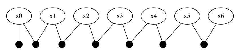
The next 6 nodes are added with odometry in an counter-clockwise hexagonal manner. Note how variables are denoted with symbols, :x2 == Symbol("x2"):
# Drive around in a hexagon
for i in 0:5
  psym = Symbol("x$i")
  nsym = Symbol("x$(i+1)")
  addVariable!(fg, nsym, Pose2)
  pp = Pose2Pose2(MvNormal([10.0;0;pi/3], Matrix(Diagonal([0.1;0.1;0.1].^2))))
  addFactor!(fg, [psym;nsym], pp )
end
At this point it would be good to see what the factor graph actually looks like:
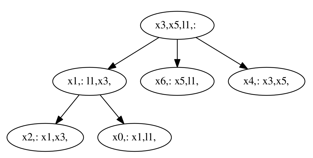
drawGraph(fg)You should see the program evince open with this visual:
Performing Inference
Let's run the multimodal-incremental smoothing and mapping (mm-iSAM) solver against this fg object:
# perform inference, and remember first runs are slower owing to Julia's just-in-time compiling
tree = solveTree!(fg)
This will take a couple of seconds (including first time compiling for all Julia processes). If you wanted to see the Bayes tree operations during solving, set the following parameters before calling the solver:
getSolverParams(fg).drawtree = true
getSolverParams(fg).showtree = true
Some Visualization Plot
2D plots of the factor graph contents is provided by the RoMEPlotting package. See further discussion on visualizations and packages here.
## Inter-operating visualization packages for Caesar/RoME/IncrementalInference exist
using RoMEPlotting

# For Juno/Jupyter style use
pl = drawPoses(fg)

# For scripting use-cases you can export the image
pl |> Gadfly.PDF("/tmp/test.pdf") # or PNG(...)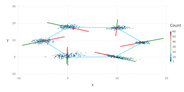
Adding Landmarks as Point2
Suppose some sensor detected a feature of interest with an associated range and bearing measurement. The new variable and measurement can be included into the factor graph as follows:
# Add landmarks with Bearing range measurements
addVariable!(fg, :l1, Point2, tags=[:LANDMARK;])
p2br = Pose2Point2BearingRange(Normal(0,0.1),Normal(20.0,1.0))
addFactor!(fg, [:x0; :l1], p2br)

# Initialize :l1 numerical values but do not rerun solver
initAll!(fg)
NOTE The default behavior for initialization of variable nodes implies the last variable node added will not have any numerical values yet, please see ContinuousScalar Tutorial for deeper discussion on automatic initialization (autoinit). A slightly expanded plotting function will draw both poses and landmarks (and currently assumes labels starting with :x and :l respectively)–-notice the new landmark bottom right:
drawPosesLandms(fg)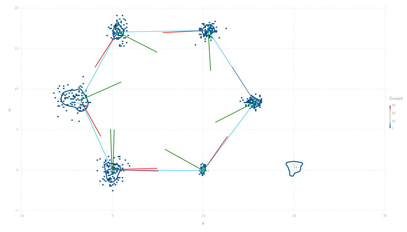
One type of Loop-Closure
Loop-closures are a major part of SLAM based state estimation. One illustration is to take a second sighting of the same :l1 landmark from the last pose :x6; followed by repeating the inference and re-plotting the result–-notice the tighter confidences over all variables:
# Add landmarks with Bearing range measurements
p2br2 = Pose2Point2BearingRange(Normal(0,0.1),Normal(20.0,1.0))
addFactor!(fg, [:x6; :l1], p2br2)

# solve
tree = solveTree!(fg, tree)

# redraw
pl = drawPosesLandms(fg)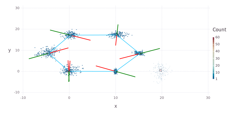
This concludes the Hexagonal 2D SLAM example.
Interest: The Bayes (Junction) tree
The Bayes (Junction) tree is used as an acyclic (has no loops) computational object, an exact algebraic refactorizating of factor graph, to perform the associated sum-product inference. The visual structure of the tree can be extracted by modifying the command tree = wipeBuildNewTree!(fg, drawpdf=true) to produce representations such as this in bt.pdf.