Data Association and Hypotheses

Ambiguous data and processing often produce complicated data association situations. In SLAM, loop-closures are a major source of concern when developing autonomous subsystems or behaviors. To illustrate this point, consider the two scenarios depicted below:

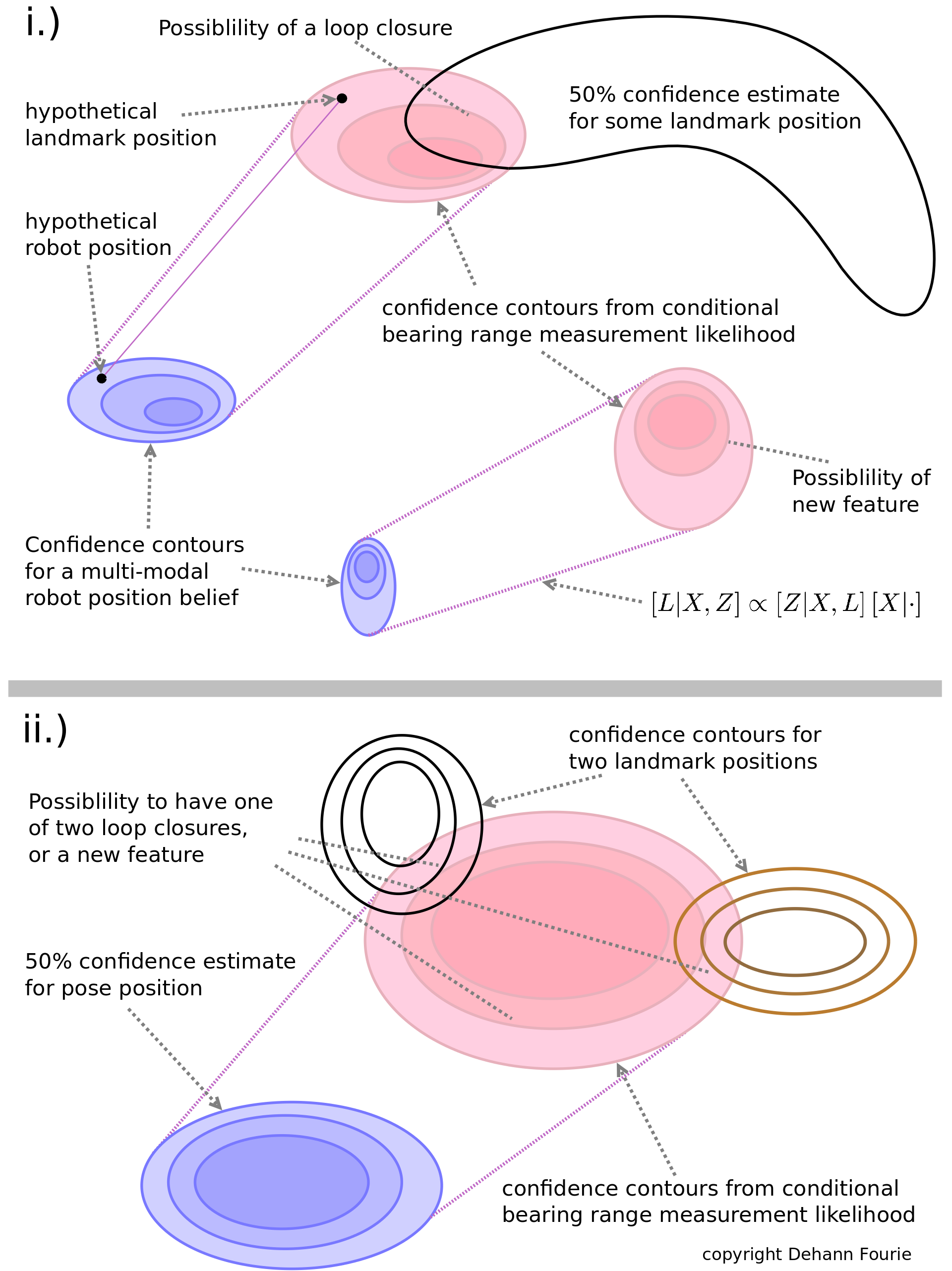
In conventional parametric Gaussian-only systems an incorrect loop-closure can occur, resulting in highly unstable numerical solutions. The mm-iSAM algorithm was conceived to directly address these (and other related) issues by changing the fundamental manner in which the statistical inference is performed.

The data association problem applies well beyond just loop-closures including (but not limited to) navigation-affordance matching and discrepancy detection, and indicates the versatility of the IncrementalInference.jl standardized multihypo interface. Note that much more is possible, however, the so-called single-fraction multihypo approach already yields significant benefits and simplicity.

Multihypothesis

Consider for example a regular three variable factor [:pose;:landmark;:calib] that due to some decision has a triple association uncertainty about the middle variable. This fractional certainty can easily be modelled via:

addFactor!(fg, [:p10, :l1_a,:l1_b,:l1_c, :c], PoseLandmCalib, multihypo=[1; 0.6;0.3;0.1; 1])

Therefore, the user can "partition" certainty about one variable using any arbitrary n-ary factor. The 100% certain variables are indicated as 1, while the remaining uncertainties regarding the uncertain data association decision are grouped as positive fractions that sum to 1. In this example, the values 0.6,0.3,0.1 represent the confidence about the association between :p10 and either of :l1_a,:l1_b,:l1_c.

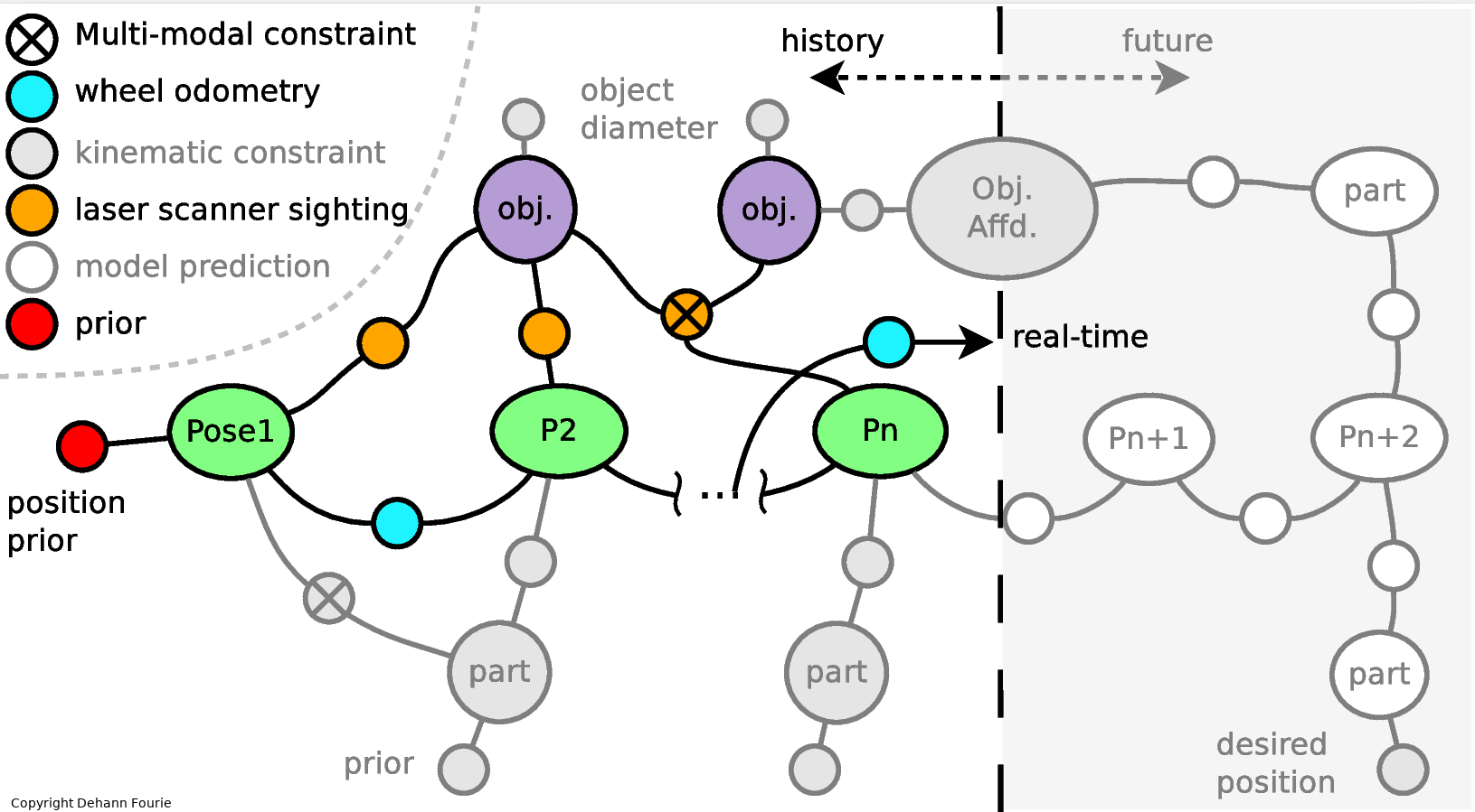
A more classical binary multihypothesis example is illustated in the multimodal (non-Gaussian) factor graph below:

Mixture Models

Mixture is a different kind of multi-modal modeling where different hypotheses of the measurement itself are unknown. It is possible to also model uncertain data associations as a Mixture(Prior,...) but this is a feature of factor graph modeling something different than data association uncertainty in n-ary factors: e.g. it is possible to use Mixture together with multihypo= and be sure to take the time to understand the different and how these concepts interact. The Caesar.jl solution is more general than simply allocating different mixtures to different association decisions. All these elements together can create quite the multi-modal soup. A practical example from SLAM is a loop-closure where a robot observes an object similar to one previously seen. The measurement observation is one thing (can maybe be a Mixture) and the association of this "measurement" with this or that variable is a multihypothesis selection.

See the familiar RobotFourDoor.jl as example as a highly simplified case using priors where these elements effectively all the same thing. Again, Mixture is something different than multihypo= and the two can be used together.

A mixture can be created from any existing prior or relative likelihood factor, for example:

mlr = Mixture(LinearRelative, 
              (correlator=AliasingScalarSampler(...), naive=Normal(0.5,5), lucky=Uniform(0,10)),
              [0.5;0.4;0.1])

addFactor!(fg, [:x0;:x1], mlr)

See a example with Defining A Mixture Relative on ContinuousScalar for more details.

struct Mixture{N, F<:AbstractFactor, S, T<:Tuple} <: AbstractFactor

# prior factor
msp = Mixture(Prior, 
              [Normal(0,0.1), Uniform(-pi/1,pi/2)],
              [0.5;0.5])

addFactor!(fg, [:head], msp, tags=[:MAGNETOMETER;])

# Or relative
mlr = Mixture(LinearRelative, 
              (correlator=AliasingScalarSampler(...), naive=Normal(0.5,5), lucky=Uniform(0,10)),
              [0.5;0.4;0.1])

addFactor!(fg, [:x0;:x1], mlr)

Raw Correlator Probability (Matched Filter)

Realistic measurement processes are based on physical process observations such as wave function interferometry or matched filtering correlation. This style of measurement is common in RADAR and SONAR systems, and can be directly incorporated in Caesar.jl since the measurement likelihood models need not be parametric. There the raw correlator output from a sensor measurement can be directly modelled and included as part of the factor algebriac likelihood probability function:

# Building a samplable likelihood, using softmax to convert intensity-energy into a pseudo-probability
rangeLikeli = AliasingScalarSampler(rangeIndex, Flux.softmax(correlatorIntensity))

# or alternatively with existing samples similar to a what a particle filter would have done
rangeLikeli = manikde!(Euclid{1}, probPoints)

# add the relative algebra, and remember you can construct your own highly non-linear factor
rangeFct = Pose2Point2Range(rangeLikeli)

addFactor!(fg, [:x8, :beacon_8], rangeFct)

Various SamplableBelief Distribution Types

Also recognize that other features like multihypo= and Mixture readily be combined with object like this rangeFct shown above. These tricks are all possible due to the multiple dispatch magic of JuliaLang, more explicitly the following is code will all return true:

IIF.AliasingScalarSampler <: IIF.SamplableBelief
IIF.Mixture <: IIF.SamplableBelief
KDE.BallTreeDensity <: IIF.SamplableBelief
Distribution.Rayleigh <: IIF.SamplableBelief
Distribution.Uniform <: IIF.SamplableBelief
Distribution.MvNormal <: IIF.SamplableBelief

One of the more exotic examples is to natively represent Synthetic Aperture Sonar (SAS) as a deeply non-Gaussian factor in the factor graph. See Synthetic Aperture Sonar SLAM. Also see the full AUV stack using a single reference beacon and Towards Real-Time Underwater Acoustic Navigation.

Null Hypothesis

Sometimes there is basic uncertainty about whether a measurement is at all valid. Note that the above examples (multihypo and Mixture) still accept that a certain association definitely exists. A null hypothesis models the situation in which a factor might be completely bogus, in which case it should be ignored. The underlying mechanics of this approach are not entirely straightforward since removing one or more factors essentially changes the structure of the graph. That said, IncrementalInference.jl employs a reasonable stand-in solution that does not require changing the graph structure and can simply be included for any factor.

addFactor!(fg, [:x7;:l13], Pose2Point2Range(...), nullhypo=0.1)

This keyword indicates to the solver that there is a 10% chance that this factor is not valid.